
Summary
The inventory cycle is the recurring alternation between periods when the growth rate of businesses’ stocks of goods rises and periods when it falls. The phase of the cycle affects comparables’ operating margins through inventory accounting. For instance, a manufacturer whose work in process and finished goods carry more fixed production overhead at the end of the year than at the beginning reports a higher margin, other things being equal, and one whose capitalized overhead falls reports a lower margin. For a comparable that uses last-in, first-out (LIFO), a reduction in inventory charges costs from older layers to cost of goods sold and raises the margin if costs have risen since those layers were added. The LIFO reserve that such a comparable discloses, if material, permits its inventory and cost of goods sold to be restated approximately to a non-LIFO basis before its margins are compared with those of other comparables. For comparables data, the length of the inventory cycle determines whether a benchmark window contains a complete cycle. We find through analysis of the economic data that a three-year window seldom captures a complete inventory cycle.
The inventory cycle and the three-year convention
Under the comparable profits method, Treas. Reg. § 1.482-5(b)(4) provides that profit level indicators should generally be derived from at least the taxable year under review and the two preceding taxable years. The regulations also identify “the effect of business cycles in the controlled taxpayer’s industry” as a circumstance that may warrant data from multiple years and list “[t]he economic condition of the particular industry, including whether the market is in contraction or expansion,” among the economic conditions to be compared in determining comparability. However, the regulations do not define a business cycle or refer to an inventory cycle. [1] Every comparable that holds goods for sale reports its inventories at each fiscal year-end, so the inventory cycle can be observed in the inventory levels reported on the comparables’ financial statements, and its length determines whether a three-year window contains a complete cycle (i.e., a complete upswing and a complete downswing).
The inventory cycle defined
Moses Abramovitz defined inventories as “the stock held by business at a given time” and inventory investment as “the net volume of goods added to, or removed from, stock during a given period.” [2] In an upswing of the inventory cycle, stocks grow faster or decline more slowly; in a downswing, they grow more slowly or decline faster. A cycle is measured from one peak to the next or from one trough to the next, and each complete cycle contains one upswing and one downswing.
In the Census Bureau’s seasonally adjusted series for total business inventories from January 1992 to August 2026, the growth-rate cycle, which is measured in the 12-month growth rate of inventories, lasted a median of 32 months (Exhibit 1). [3]

A comparable’s balance sheet reports inventories at the end of each fiscal year, so the percentage change from one year-end balance to the next is the comparable’s inventory growth for the year, and a series of those changes constitutes its growth-rate cycle observed at annual intervals. [4]
The inventory cycle in the financial statements
The phase of the inventory cycle affects a comparable’s reported operating margin through the accounting for inventory costs. As a result, two manufacturing comparables with the same sales and production costs can report different margins in the same year if one is adding to its inventory and the other is reducing it. For fixed overhead and for LIFO inventory, the direction of the effect depends on whether inventory increases or decreases during the year (Exhibit 2).
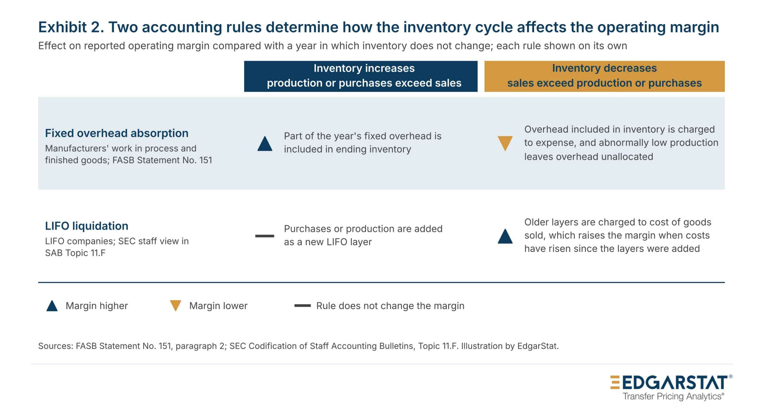
Under U.S. generally accepted accounting principles (GAAP), a manufacturer allocates fixed production overhead to inventory based on “the normal capacity of the production facilities,” and “[u]nallocated overheads are recognized as an expense in the period in which they are incurred.” [5] In a year when production exceeds sales, part of the year’s fixed overhead is included in ending inventory, and the amount by which the fixed overhead incurred exceeds the fixed overhead charged to expense equals the increase in fixed overhead carried in inventory. In a year when a manufacturer reduces its stocks, the overhead included in the inventory it sells is charged to expense, and if production is below the range of normal capacity, the overhead left unallocated is charged as well. The rule applies to the work in process and finished goods of manufacturers; wholesalers and retailers, which buy finished goods, do not allocate production overhead, and the LIFO rule described below applies to them as to manufacturers.
Exhibit 3 applies these rules to a hypothetical manufacturer whose selling price, units sold, variable cost per unit, and total fixed overhead remain unchanged for three years. Its operating margin is 17.3 percent in the year it adds 200,000 units to inventory and 10.7 percent in the year it sells them, compared with 14 percent in a year of balanced production. The margin over the three years is 14 percent because inventory is zero at the beginning and end of the period, so all $30 million of fixed overhead incurred is charged to expense. By contrast, a two-year window containing only the balanced year and the year in which inventory increases would report 15.7 percent.

Exhibit 4 records Years 2 and 3 as journal entries. In Year 2, $1.67 million of the year’s $10 million of fixed overhead is included in ending inventory, so cost of goods sold includes the remaining $8.33 million; in Year 3, that $1.67 million is charged to cost of goods sold, together with the $8.0 million allocated to the year’s production and the $2.0 million left unallocated because production was below normal capacity.

A decline in inventory quantity has a different effect on comparables that use last-in, first-out (LIFO). When a LIFO company reduces its inventory, costs from older layers (quantities added in earlier years and recorded at those years’ costs) are charged to cost of goods sold. If costs have risen since those layers were added, the reduction raises the year’s margin. The Securities and Exchange Commission (SEC) staff view is that disclosure of “the amount of income realized as a result of the inventory liquidation” is required when a substantial liquidation adds a material amount of income. [6] LIFO comparables also disclose, if material, the excess of replacement or current cost over the LIFO carrying amount. Compustat collects this amount, when disclosed, as LIFO Reserve (LIFR), so the inventory and cost of goods sold of a LIFO comparable can be restated approximately to a non-LIFO basis before its margins are compared with those of first-in, first-out (FIFO) comparables. On that basis, inventory is approximately Inventories, Total (INVT) plus LIFR, and cost of goods sold is approximately Cost of Goods Sold (COGS) less the year’s increase in LIFR. [7]
The regulations treat these differences as a question of reliability: under Treas. Reg. § 1.482-5(c)(3)(ii), “if differences in inventory and other cost accounting practices would materially affect operating profit, the ability to make reliable adjustments for such differences would affect the reliability of the results.” When the profit level indicator is the rate of return on capital employed, “the ratio of operating profit to operating assets,” the inventory cycle can affect both terms because the accounting rules described above change operating profit as inventory rises and falls, and operating assets include inventories, measured as the average of their values at the beginning and the end of the year. [8]
The length of the review window and the length of the cycle
Writers from 1923 to 1941 described a short cycle of about 40 months, and Alvin Hansen, in 1941, attributed these minor fluctuations, most lasting 3 or 4 years, primarily to inventory investment. [9]
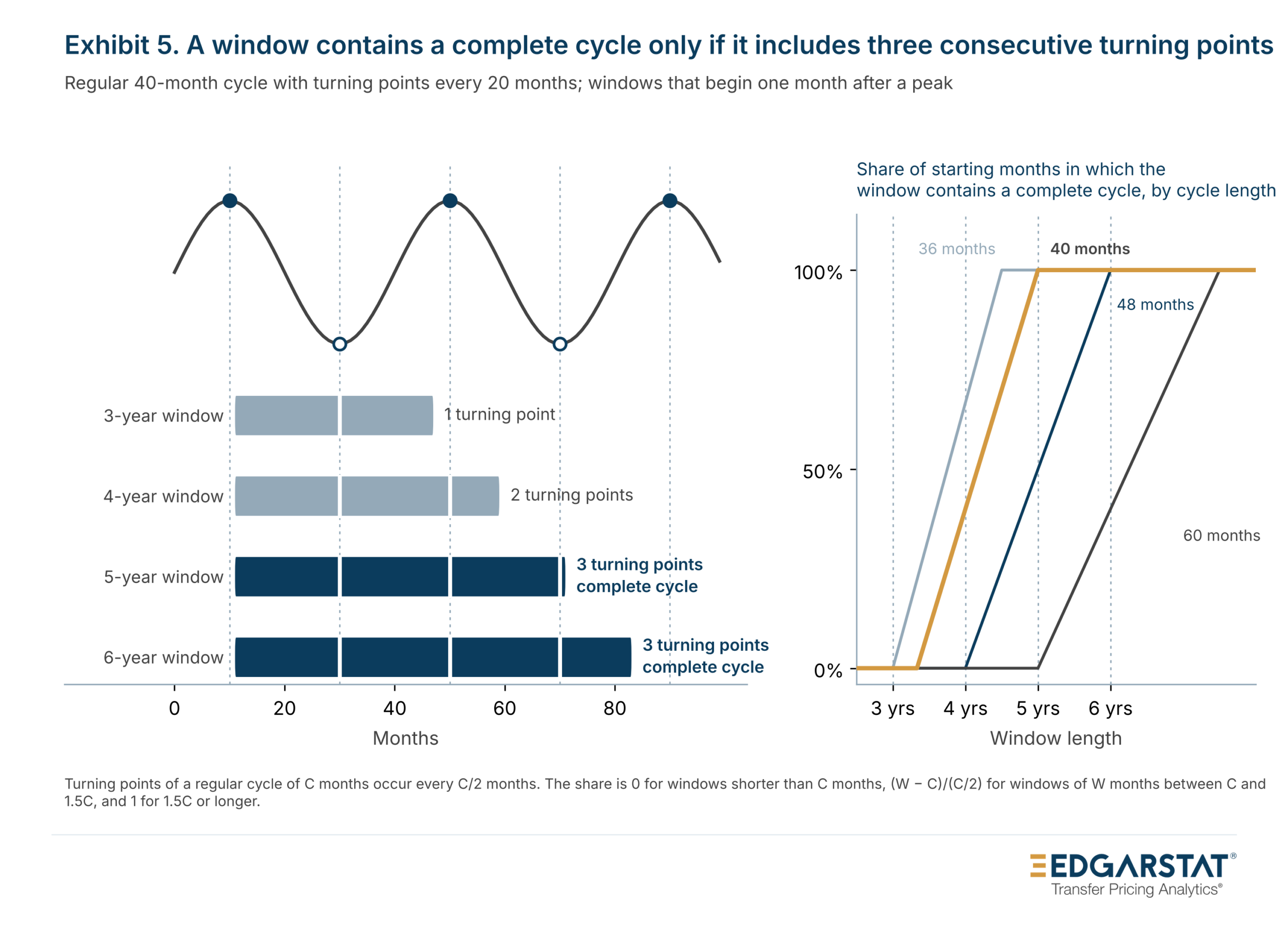
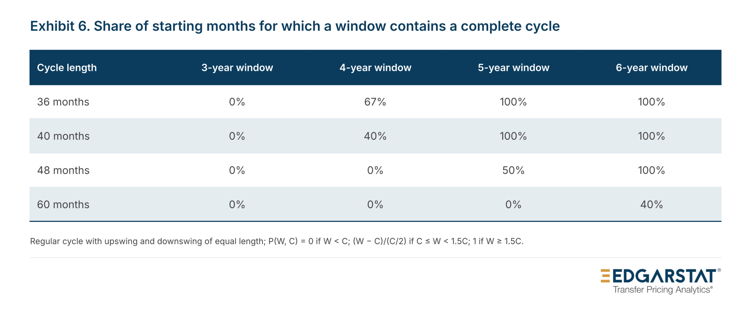
A window of years contains a complete cycle only if three consecutive turning points fall within it. A three-year window does not contain a complete cycle of 36 months or longer for any starting month (Exhibits 5 and 6). For the 40-month cycle described in earlier literature, with an upswing and a downswing of equal length, a four-year window contains a complete cycle for 40 percent of starting months, and a five-year window contains one for every starting month. Because actual cycles are irregular, the share of windows that contain a complete cycle must be measured using dated turning points. [10]
Future entries in this series will examine how often benchmark windows of different lengths contain a complete inventory cycle in industry data and in the financial statements of comparables.
Endnotes
- Treas. Reg. § 1.482-5(b)(4) provides that profit level indicators “should be derived from a sufficient number of years of data to reasonably measure returns that accrue to uncontrolled comparables,” that “[g]enerally, such a period should encompass at least the taxable year under review and the preceding two taxable years,” and that the analysis “must be applied in accordance with § 1.482-1(f)(2)(iii)(D).” Section 1.482-1(f)(2)(iii)(B) provides that the extent to which multiple-year data are appropriate “depends on the method being applied and the issue being addressed” and that such data “must ordinarily be considered” in applying the comparable profits method; it also provides that they “ordinarily will not be considered” in applying the comparable uncontrolled price method except where risk or market share strategy issues are present. Section 1.482-1(d)(3)(iv) provides that determining the degree of comparability “requires a comparison of the significant economic conditions that could affect the prices that would be charged or paid, or the profit that would be earned in each of the transactions,” and paragraph (d)(3)(iv)(G) lists among those factors “[t]he economic condition of the particular industry, including whether the market is in contraction or expansion.” Section 1.482-5(c)(2)(i) lists “the stage in a business or product cycle” among the facts and circumstances on which comparability depends. Section 1.482-1(f)(2)(iii)(A) provides that if multiple-year data are used for the comparables, “data relating to the controlled taxpayer for the same years ordinarily must be considered,” and that if such data are not available, “reliable data from other years, as adjusted under paragraph (d)(2)” may be used. Section 1.482-1(f)(2)(iii)(C) provides that data from multiple years “may be considered to determine whether the same economic conditions that caused the controlled taxpayer’s results had a comparable effect over a comparable period of time on the uncontrolled comparables that establish the arm’s length range”; it adds that “persistent losses among controlled taxpayers may be an indication of non-arm’s length dealings,” so that where a controlled taxpayer seeks to demonstrate that a loss is within the arm’s length range, the district director “may take into account data from taxable years other than the taxable year of the transaction.” In Example 3 of § 1.482-1(f)(2)(iii)(E), which illustrates paragraph (C), a distributor realizes losses on its controlled transactions in each of five consecutive taxable years, and in each year a different uncontrolled comparable realizes a loss equal to or greater than the distributor’s; because each comparable realized a loss in only one of the five years and their average result over the five years was a profit, the district director “may conclude that the controlled taxpayer’s results are not within the arm’s length range over the five year period.” The eCFR text of the example refers to “paragraph (f)(3)(iii)(C) of this section,” which appears to be a misreference to paragraph (f)(2)(iii)(C). Section 1.482-1(f)(2)(iii)(D) provides that where comparing average results over the same multiple-year period “would reduce the effect of short-term variations that may be unrelated to transfer pricing, it may be appropriate to establish a range derived from the average results of uncontrolled comparables over a multiple year period.” An adjustment in that case “ordinarily will be equal to the difference, if any, between the controlled taxpayer’s result for the taxable year and the mid-point of the uncontrolled comparables’ results for that year,” is ordinarily made to the median where the interquartile range is used and is made “only to the extent that it would move the controlled taxpayer’s multiple year average closer to the arm’s length range for the multiple year period or to any point within such range.” Example 1 of § 1.482-1(f)(2)(iii)(E) applies the resale price method and averages the comparables’ results over the years 1993 to 1995 to account for “cyclical factors.” The final regulations in §§ 1.482-1 to 1.482-9 do not define a business cycle or refer to an inventory cycle, and they do not state a maximum number of years. The eCFR text of § 1.482-1(j)(1) reads “The regulations in this are generally effective for taxable years beginning after October 6, 1994,” with a word omitted. Section 1.482-5 does not contain its own effective-date paragraph; its source note cites T.D. 8552, 59 FR 35021, July 8, 1994. Section 1.482-1(j)(6)(i) provides that paragraph (f)(2)(iii)(B) is “generally applicable for taxable years beginning after July 31, 2009,” and § 1.482-1(j)(6)(ii) permits an election to apply it to earlier taxable years. Regulation text is from the eCFR as of October 1, 2026.
- Moses Abramovitz, Inventories and Business Cycles, with Special Reference to Manufacturers’ Inventories (NBER, 1950), p. 4, note 1.
- U.S. Census Bureau, Manufacturing and Trade Inventories and Sales, total business inventories, seasonally adjusted, millions of current dollars, January 1992 to August 2026, from the Business and Industry Time Series database file updated October 15, 2026. The Bureau values inventories at cost and reports manufacturers’ and retailers’ inventories on a basis other than last-in, first-out (LIFO). It notes for retailers that “[m]ethods of valuation may vary according to the accounting practices of each firm,” and its wholesale definition states only that inventories are valued at cost (U.S. Census Bureau, “Manufacturing & Trade Inventories & Sales: Definitions” and “Wholesale Trade: Definitions”). Because the series is in current dollars, its changes include changes in the cost of goods held as well as changes in quantities. The dollar level declined for seven months or longer in three episodes, each of which overlapped a recession dated by the National Bureau of Economic Research (NBER); the largest, 14.6 percent from August 2008 to September 2009, overlapped the recession that the NBER dates from December 2007 to June 2009. The other two declines in the level, 7.7 percent from January 2001 to April 2002 and 6.1 percent from November 2019 to June 2020, overlapped the recessions dated from March to November 2001 and from February to April 2020 (NBER, “US Business Cycle Expansions and Contractions”). The level also declined for four months, by 1.3 percent from April to August 2003 and by 0.7 percent from October 2015 to February 2016. The 12-month growth rate was lowest, at minus 14.1 percent, in August 2009 and highest, at 21.7 percent, in June 2022. Turning points are dated with a modified version of the rules of Gerhard Bry and Charlotte Boschan, Cyclical Analysis of Time Series: Selected Procedures and Computer Programs (NBER, 1971), ch. 2: a peak (trough) is the highest (lowest) value within five months on either side, peaks and troughs alternate, cycles last at least 15 months and phases last at least five months. The smoothing stages of the procedure and its end-of-series rules are not applied; a turning point is identified only where five months of data exist on either side of it.
- The change in the year-end balance also includes the effects of acquisitions, currency translation, write-downs and, for a company that uses LIFO, the LIFO method. Because inventories are carried at cost, the change in the balance is a change in book value and also reflects changes in the cost of goods held. Annual changes provide observations from which turning points can be estimated; they do not recover every monthly turning point, and a short annual series does not by itself establish that the cycle recurs.
- FASB Statement No. 151, Inventory Costs, an amendment of ARB No. 43, Chapter 4 (November 2004), paragraph 2, which amends paragraph 5 and footnote 2 of ARB 43, Chapter 4; the amended text includes paragraph 5A. Statement 151 also provides that “[n]ormal capacity refers to a range of production levels,” that “[j]udgment is required to determine when a production level is abnormally low (that is, outside the range of expected variation in production),” that “[t]he actual level of production may be used if it approximates normal capacity,” that “[i]n periods of abnormally high production, the amount of fixed overhead allocated to each unit of production is decreased so that inventories are not measured above cost,” and that “[t]he amount of fixed overhead allocated to each unit of production is not increased as a consequence of abnormally low production or idle plant.” Its provisions “shall be effective for inventory costs incurred during fiscal years beginning after June 15, 2005” and “shall be applied prospectively,” and “[e]arlier application is permitted for inventory costs incurred during fiscal years beginning after the date this Statement is issued.” The amended text provides that “the allocation of fixed production overheads to the costs of conversion is based on the normal capacity of the production facilities,” so the margin effect described in the body depends on the change in fixed production overhead carried in work in process and finished goods, other things being equal; because raw materials have not been converted, an increase in raw materials alone does not defer the manufacturer’s own production overhead. The quotations are the text of Statement 151, and the paragraph of the FASB Accounting Standards Codification that now contains this guidance was not verified for this post.
- SEC, Codification of Staff Accounting Bulletins, Topic 11.F, “LIFO Liquidations.” The facts address a registrant that “liquidates a substantial portion of its LIFO inventory and as a result includes a material amount of income in its income statement which would not have been recorded had the inventory liquidation not taken place.” The staff’s response is that disclosure “would be required in order to make the financial statements not misleading” and “may be made either in a footnote or parenthetically on the face of the income statement.”
- Regulation S-X, 17 CFR 210.5-02, caption 6(c), text from the eCFR as of October 1, 2026: “If the LIFO inventory method is used, the excess of replacement or current cost over stated LIFO value shall, if material, be stated parenthetically or in a note to the financial statements.” The non-LIFO basis is the basis against which the company measures its LIFO reserve, and the change in LIFR can also include the effects of acquisitions and currency translation. The Advance Pricing Agreement Program’s “Compustat Tools for Transfer Pricing Analysis” (March 5, 1998) describes the same adjustment, stating that “[n]ormally, accountants adjust cost of goods sold (COGS) by subtracting the difference between the year-end LIFO reserve and the year-beginning LIFO reserve,” and its tool adjusts average inventory by adding the average LIFO reserve; the tool offers an option to assume that the difference is zero when the data are unavailable, which this post does not adopt. When a comparable does not disclose a quantified reserve, the adjustment cannot be calculated, and a missing LIFR value should not be read as zero; Compustat’s definition of LIFR was not compared with the Regulation S-X caption for this post.
- Treas. Reg. § 1.482-5(c)(3)(ii). The resale price and cost plus methods contain the same sentence with respect to the gross profit margin and the gross profit markup, in § 1.482-3(c)(3)(iii)(B) and (d)(3)(iii)(B), and § 1.482-3(c)(3)(ii)(C) lists “[i]nventory levels and turnover rates, and corresponding risks, including any price protection programs offered by the manufacturer” among the factors that may be particularly relevant to the resale price method. Section 1.482-5(b)(4)(i) defines the rate of return on capital employed as “the ratio of operating profit to operating assets” and provides that its reliability “depends on the extent to which the composition of the tested party’s assets is similar to that of the uncontrolled comparable.” Section 1.482-5(d)(6) defines operating assets as “the value of all assets used in the relevant business activity of the tested party, including fixed assets and current assets (such as cash, cash equivalents, accounts receivable, and inventories),” excludes “investments in subsidiaries, excess cash, and portfolio investments,” permits measurement “by their net book value or by their fair market value, provided that the same method is consistently applied to the tested party and the comparable parties, and consistently applied from year to year,” provides that “it may be necessary to take into account recent acquisitions, leased assets, intangibles, currency fluctuations, and other items that may not be explicitly recorded in the financial statements,” and requires the average of the values for the beginning and the end of the year “unless substantial fluctuations in the value of operating assets during the year make this an inaccurate measure of the average value over the year,” in which case “a more accurate measure of the average value of operating assets must be applied.” For a domestic tested party, the controlled taxpayer whose results are compared with those of the comparables, the tax-basis counterparts of the comparables’ inventory data are reported on its own Form 1125-A, Cost of Goods Sold (Rev. November 2024), when that form is available. Lines 1 and 7 report inventory at the beginning and at the end of the year, so the change in the tested party’s tax-basis inventory for the year is equal to line 7 less line 1; line 9b asks whether there was a writedown of subnormal goods, and for a LIFO taxpayer, line 9d(ii) reports the closing LIFO reserve. Form 1125-A includes additional § 263A costs on line 4, so tax-basis inventory can differ from the inventory reported in the financial statements, and the instructions for line 1 require a taxpayer that changes its method of accounting to “refigure last year’s closing inventory using the new method of accounting.” Under 26 U.S.C. § 472(c), the use of LIFO permitted by § 472(a) is available only if the taxpayer establishes to the satisfaction of the Secretary that it has not used any procedure other than LIFO in inventorying the goods “to ascertain the income, profit, or loss of the first taxable year for which the method described in subsection (b) is to be used, for the purpose of a report or statement covering such taxable year” either “to shareholders, partners, or other proprietors, or to beneficiaries” or “for credit purposes”; § 472(e)(2) permits the Secretary to require a change of method if another procedure is used for such a report or statement for a later taxable year. Section 472(g)(1) provides that “[e]xcept as otherwise provided in regulations, all members of the same group of financially related corporations shall be treated as 1 taxpayer for purposes of subsections (c) and (e)(2),” and § 472(g)(2) defines that group as “any affiliated group as defined in section 1504 determined by substituting ’50 percent’ for ’80 percent’ each place it appears in section 1504(a) and without regard to section 1504(b)” and “any other group of corporations which consolidate or combine for purposes of financial statements.”
- Joseph A. Schumpeter, Business Cycles: A Theoretical, Historical, and Statistical Analysis of the Capitalist Process, vol. 1 (McGraw-Hill, 1939), p. 165 and note 1, p. 169 and note 1, and p. 215. Schumpeter gives the title of Kitchin’s article, “Cycles and Trends in Economic Factors,” on p. 215, and on p. 165, note 1, he cites the two studies as published in the Review of Economic Statistics for January 1923, “preliminary vol. V, pp. 17 et seq, and p. 10 et seq,” and quotes Crum’s caveat. The two 1923 articles are cited as Schumpeter describes them. According to Schumpeter, Crum found “a period of roughly 40 months” in monthly commercial paper rates in New York from 1866 to 1922, and Kitchin found the same cycle “in bank clearings and wholesale prices, as well as in interest rates, for both Great Britain and the United States, during the period 1890 to 1922.” Schumpeter named the short cycle after Kitchin and described it as a cycle that “is not exactly or even modally just 40 months,” and Crum wrote of his own result that “the economic period should not be assumed constant.” None of the series in which Crum and Kitchin found the cycle is a measure of inventories, and none of these early estimates of its length was made for an individual industry. Hansen’s attribution is reported in Abramovitz, Inventories and Business Cycles, p. 23, describing Alvin H. Hansen, Fiscal Policy and Business Cycles (Norton, 1941): Hansen distinguished “minor” fluctuations “most of which last 3 or 4 years” and attributed them “primarily to fluctuations in inventory investment.” Hansen’s book is cited as Abramovitz describes it. On p. 494, Abramovitz writes that Hansen believes the minor cycles are caused “not infrequently” by fluctuations in inventory investment. The business cycles dated by the NBER from 1945 to 2020 averaged 74.5 months from trough to trough, compared with 48.2 and 53.2 months for 1854 to 1919 and 1919 to 1945, respectively (NBER, “US Business Cycle Expansions and Contractions,” average duration table).
- The turning points of a regular cycle of C months occur every C/2 months, so a window contains three of them for every starting month only if it is at least 1.5C months long, and for no starting month if it is shorter than C months. For a window of W months between those lengths, the share of starting months for which it contains three turning points is (W − C)/(C/2). The calculation assumes an upswing and a downswing of equal length and a window of W months that contains W monthly observations. For a 40-month cycle with a 30-month upswing and a 10-month downswing, a five-year window contains a complete cycle for 75 percent of starting months, and a window of 70 months is needed for every starting month. The criterion of three consecutive dated turning points identifies a window that contains a complete dated cycle; a window exactly one period long that begins and ends between turning points includes every phase of a regular cycle but contains only two turning points. The calculation establishes how often a window contains a complete dated cycle. It does not by itself establish that a window of a given length removes the accounting effects of the cycle from a benchmark, because a complete growth-rate cycle does not require the closing balances of inventory and of capitalized overhead to equal the opening balances; in Exhibit 3, the three-year margin equals the margin of the balanced year because inventory is zero at the beginning and at the end of the three years.