
1. The question
The Travelled Road closed with a protocol of six steps. Step five instructs the analyst to publish, for each company-year, the leverage h(i,t) and the factor 1/[1-h(i,t)]^2, so that the reader sees which companies widen the interval. Publication answers the question which. It does not answer the question how much is too much. This note supplies the boundaries, and in doing so separates three concepts that practitioner reports tend to merge: the distance of a company-year in the regressor (leverage), its effect on the estimated slope (influence), and the unit at which a comparable enters the sample (the company, not the company-year).
The model is the one of the earlier post. Revenue R (Compustat REVT) is regressed on operating cost X (XOPR) across n companies and T years, N = nT company-years, with p = 2 parameters:
\quad
(1)\qquad
R(i,t) = \lambda_0 + \lambda_1 X(i,t) + \varepsilon(i,t), \qquad
\operatorname{Var}[\varepsilon(i,t)] = \sigma^2(i,t).
The errors are independent with unequal variances. The slope estimate is b_1 = \sum x(i,t)R(i,t)/S_{xx}, where x(i,t) is the deviation of X(i,t) from its mean and S_{xx} = \sum x(i,t)^2. The example sample remains n = 8, T = 3, N = 24.
2. What leverage measures
Leverage is the diagonal element of the hat matrix H = X(X'X)^{-1}X'. In the bivariate model it reduces to
\quad
(2)\qquad
h(i,t) = \frac{1}{N} + \frac{x(i,t)^2}{S_{xx}}.
Its meaning follows from the fitted values. Since \hat R = HR, each fitted value is a weighted sum of all observed revenues, and h(i,t) is the weight a company-year places on its own revenue:
\quad
(3)\qquad
\hat R(i,t) = h(i,t)\,R(i,t) + \sum_{(j,s)\neq(i,t)} H_{(i,t),(j,s)}\,R(j,s).
Three properties follow. First, 1/N \le h(i,t) \le 1. Second, the leverages sum to the number of parameters, \sum h(i,t) = p = 2, so the average is p/N. Third, writing s^2 = S_{xx}/N and z(i,t) = x(i,t)/s for the standardized distance of operating cost from its mean,
\quad
(4)\qquad
h(i,t) = \frac{1 + z(i,t)^2}{N}.
Leverage is a function of X alone. It is fixed before any revenue is observed. A boundary on h is therefore a boundary on the design of the sample, not on its outcome, a distinction to which Section 7 returns.
3. How leverage enters the HC3 variance
The ordinary residual understates the error where leverage is high, because E[e(i,t)^2] = \sigma^2(i,t)[1 - h(i,t)]. HC3 replaces the residual by the deleted residual d(i,t) = e(i,t)/[1-h(i,t)], so that V_3(b_1) = \sum x^2 d^2/S_{xx}^2. The factor 1/[1-h]^2 is the price HC3 charges for distance. The deletion formulas of Belsley, Kuh and Welsch (1980), restated for computation by Velleman and Welsch (1981), give the change in the slope when company-year (i,t) is removed from the fit:
\quad
(5)\qquad
\Delta(i,t) = b_1 - b_1(-it) = \frac{x(i,t)\,d(i,t)}{S_{xx}}.
Squaring and summing (5) over the sample yields an identity that organizes the rest of this note:
\quad
(6)\qquad
V_3(b_1) = \sum_{i,t} \Delta(i,t)^2.
The HC3 variance of the slope is the sum of the squared changes in the slope produced by deleting each company-year in turn. This is the bridge between HC3 and the jackknife, and it supplies a measure of influence stated in the same units as the reported interval. Define the share of company-year (i,t) in the HC3 variance:
\quad
(7)\qquad
c(i,t) = \frac{\Delta(i,t)^2}{V_3(b_1)} = \frac{x(i,t)^2 d(i,t)^2}{\sum x^2 d^2}, \qquad \sum c(i,t) = 1.
Under equal contribution each company-year would hold the proportional share 1/N.
4. Boundaries on leverage
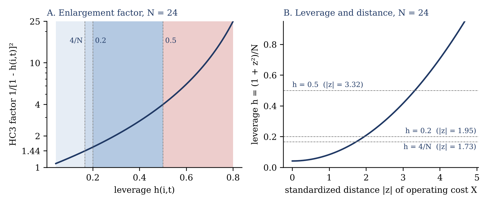
The relative boundary. Hoaglin and Welsch (1978) treat h > 2p/N as high leverage, twice the average. With p = 2 the boundary is 4/N, and by (4) it is equivalent to |z| > \sqrt{3} \approx 1.73 for every N. In words: a company-year is high-leverage when its operating cost lies more than 1.73 standard deviations from the sample mean. At the boundary the HC3 factor is [N/(N-4)]^2, which equals 1.44 at N = 24.
The absolute boundaries. Huber (1981) grades leverage on a fixed scale: h \le 0.2 is safe, 0.2 < h \le 0.5 is risky, and h > 0.5 is to be avoided. The ceiling of 0.5 has a direct reading in (3): above it, a company-year supplies more than half of its own fitted value. Its expected squared residual is less than half its error variance, its deleted residual exceeds twice its residual, and its HC3 factor exceeds 4. The regression no longer tests that company-year; the company-year dictates the regression at that point.
A coincidence worth noting. Cribari-Neto (2004) proposed HC4, which replaces the exponent 2 of HC3 by \delta(i,t) = \min\{4,\, N h(i,t)/p\}. The exponent exceeds 2 if and only if h(i,t) > 2p/N. The Hoaglin–Welsch boundary is therefore the point at which HC4 judges the HC3 correction insufficient. The two literatures, one on diagnostics and one on covariance estimation, place the first boundary at the same value.
| Grade | Boundary | |z| at N = 24 | Factor 1/(1 − h)² | Reading |
|---|---|---|---|---|
| Tolerable | h \le 2p/N = 4/N | ≤ 1.73 | ≤ 1.44 | Within twice the average leverage |
| High | 4/N < h \le 0.2 | 1.73 to 1.95 | 1.44 to 1.56 | Hoaglin–Welsch high; Huber safe |
| Severe | 0.2 < h \le 0.5 | 1.95 to 3.32 | 1.56 to 4.00 | Huber risky; HC4 exponent above 2 |
| Intolerable | h > 0.5 | > 3.32 | > 4.00 | Own revenue sets most of own fit |
5. Leverage is not influence
A company-year far from the mean of X that lies on the regression line contributes to the precision of the estimate: it lengthens the lever arm and reduces the variance of the slope. Its deleted residual is small, so its \Delta(i,t) is small despite a large factor. Distance becomes a problem only in combination with a residual. Influence is the product, and (5) measures it: x(i,t) carries the distance, d(i,t) carries the leverage-corrected residual.
Belsley, Kuh and Welsch (1980) flag a scaled coefficient change above 2/\sqrt{N}. Their scaling uses a common error variance, which the premise of HC3 rejects. Restated in HC3 units, |\Delta(i,t)|/\mathrm{SE}_3(b_1) = \sqrt{c(i,t)}, and the Belsley–Kuh–Welsch boundary becomes
\quad
(8)\qquad
c(i,t) > 4/N.
A company-year is influential when it supplies more than four times its proportional share of the HC3 variance. Identity (6) adds a second fact: since c(i,t) \le 1, no single company-year can move the slope by more than one HC3 standard error. A company-year can, however, own the interval. We propose c(i,t) > 1/2 as intolerable: one company-year then contributes most of the uncertainty that the report b_1 \pm \mathrm{SE}_3(b_1) attributes to the sample.
6. The company as the unit
The Travelled Road conceded that HC3 treats the T years of one company as independent, which they are not. The same accounting policies, the same scale, and the same product mix recur from one year to the next. A company with three high-leverage years enters the regression as one large comparable observed three times. MacKinnon, Nielsen and Webb (2023) develop measures of leverage and influence at the level of the cluster; with the company as the cluster, the company leverage is the trace of its diagonal block of H:
\quad
(9)\qquad
H(i) = \sum_t h(i,t), \qquad \sum_i H(i) = p, \qquad \text{average } p/n.
By analogy with Hoaglin and Welsch, a company is high-leverage when H(i) > 2p/n. At n = 8 the boundary is 0.5, a quarter of the total leverage of the sample held by one of eight companies. The change in the coefficients when the whole company is removed follows from the block deletion formula:
\quad
(10)\qquad
b - b(-i) = (X'X)^{-1} X_i' \,[I_T - H_{ii}]^{-1} e_i,
where X_i, H_{ii} and e_i are the rows, diagonal block and residuals of company i. Let \Delta(i) denote the slope element of (10). Unlike the company-year shift, \Delta(i) is not bounded by \mathrm{SE}_3: shifts of the same sign in T years accumulate. Two boundaries follow. A company is flagged when |\Delta(i)|/\mathrm{SE}_3 > 2/\sqrt{n}, the Belsley–Kuh–Welsch scaling applied to n companies. A company is intolerable when
\quad
(11)\qquad
\frac{|\Delta(i)|}{\mathrm{SE}_3(b_1)} > 1,
because its removal then moves the slope outside the reported one-standard-error interval, and b_1 \pm \mathrm{SE}_3(b_1) describes that company rather than the sample. The extreme case occurs when I_T - H_{ii} is singular: the slope is then not identified without company i, and the comparable set is one company with satellites.
| n (T = 3) | N | 4/N | Factor at 4/N | |z| at h = 0.5 | c(i,t) flag 4/N | H(i) flag 2p/n | Δ(i) flag 2/√n |
|---|---|---|---|---|---|---|---|
| 8 | 24 | 0.167 | 1.44 | 3.32 | 0.167 | 0.500 | 0.71 |
| 10 | 30 | 0.133 | 1.33 | 3.74 | 0.133 | 0.400 | 0.63 |
| 15 | 45 | 0.089 | 1.20 | 4.64 | 0.089 | 0.267 | 0.52 |
| 20 | 60 | 0.067 | 1.15 | 5.39 | 0.067 | 0.200 | 0.45 |
7. What to do with an intolerable comparable
The protocol of The Travelled Road removes no company by rank, and the boundaries above do not license removal by rank under another name. An intolerable grade is a demand for examination, in three steps.
Verify the data. A company-year at extreme leverage is often an accounting event rather than an economic one: an acquisition or divestiture, a restatement, a change of fiscal year, a segment reclassification, or a currency translation. Compustat records the consolidated entity, and a consolidation event can place one year of a comparable far from its other years.
Report both estimates. State b_1 \pm \mathrm{SE}_3(b_1) with and without the intolerable company, together with the reason for the grade. The reader then judges whether the arm’s-length inference survives the company or depends on it.
Distinguish selection on X from selection on R. Exclusion based on leverage alone conditions on the regressor. The orthogonality E[\varepsilon \mid X] = 0 holds in the retained sample, and the slope remains unbiased. Exclusion based on residuals, or on the rank of a profit ratio, conditions on revenue and biases the slope; this is the defect of the interquartile range under Treas. Reg. §1.482-1(e)(2)(iii)(C). Exclusion on X is not costless, however: it narrows the range of operating cost the comparables represent. The tested party must lie inside the retained range. Its own leverage, h_0 = 1/N + x_0^2/S_{xx}, obeys the same boundaries; a tested party with h_0 > 0.5 is an extrapolation, whatever the quality of the comparables.
8. Instruction to the Kraków developers
Per company-year, publish: R, X, z, h, 1/(1-h)^2, e, d, \Delta, c, and a grade code.
- T tolerable: h \le 2p/N and c \le 4/N
- L high leverage, not influential: h > 2p/N and c \le 4/N
- I influential: c > 4/N
- X intolerable: h > 0.5 or c > 1/2
Per company, publish: H(i), \Delta(i), |\Delta(i)|/\mathrm{SE}_3, and a flag: F if H(i) > 2p/n or |\Delta(i)|/\mathrm{SE}_3 > 2/\sqrt{n}; X if |\Delta(i)|/\mathrm{SE}_3 > 1 or I_T - H_{ii} is singular.
Summary row: n, T, N, p, b_1, \mathrm{SE}_3(b_1), the boundaries 2p/N, 4/N, 2p/n, 2/\sqrt{n}, and the tested-party leverage h_0.
Check: \sum h = 2, \sum c = 1, and \sum \Delta^2 = V_3(b_1) to machine precision. Compute (5) and (10) from the identities; do not refit N + n regressions.
The boundaries do not decide the arm’s-length range. They decide which parts of the evidence the reader must examine before accepting it. The interval b_1 \pm \mathrm{SE}_3(b_1) belongs to the sample only when no company owns it.
References
Belsley, D. A., E. Kuh, and R. E. Welsch (1980). Regression Diagnostics: Identifying Influential Data and Sources of Collinearity. New York: John Wiley & Sons. Source of the deletion formulas and of the 2/\sqrt{N} boundary on scaled coefficient changes; written at the NBER Computer Research Center for econometric practice.
Cribari-Neto, F. (2004). Asymptotic inference under heteroskedasticity of unknown form. Computational Statistics & Data Analysis 45(2): 215–233. doi:10.1016/S0167-9473(02)00366-3. Introduces HC4, whose exponent \min\{4, Nh/p\} exceeds 2 above the Hoaglin–Welsch boundary.
Davidson, R., and J. G. MacKinnon (2004). Econometric Theory and Methods. New York: Oxford University Press. Section 2.6 treats leverage and influential observations; Chapter 5 treats heteroskedasticity-robust covariance estimators.
Hoaglin, D. C., and R. E. Welsch (1978). The hat matrix in regression and ANOVA. The American Statistician 32(1): 17–22. Source of the 2p/N boundary.
Huber, P. J. (1981). Robust Statistics. New York: John Wiley & Sons. Second edition, with E. M. Ronchetti, 2009. Source of the absolute grades 0.2 and 0.5.
MacKinnon, J. G., M. Ø. Nielsen, and M. D. Webb (2023). Leverage, influence, and the jackknife in clustered regression models: Reliable inference using summclust. The Stata Journal 23(4): 942–982. doi:10.1177/1536867X231212433. Cluster-level leverage, partial leverage and influence; the basis of Section 6.
MacKinnon, J. G., and H. White (1985). Some heteroskedasticity-consistent covariance matrix estimators with improved finite sample properties. Journal of Econometrics 29(3): 305–325. Introduces HC3.
Silva, E. A. (2026). The travelled road. EdgarStat blog, November 16, 2026. https://edgarstat.com/blog/the-travelled-road/. The protocol whose fifth step this note completes.
U.S. Treasury Regulations, 26 C.F.R. §1.482-1(e)(2)(iii)(C). Interquartile range as the arm’s-length range under statistical methods.
Velleman, P. F., and R. E. Welsch (1981). Efficient computing of regression diagnostics. The American Statistician 35(4): 234–242. doi:10.1080/00031305.1981.10479362. Computing formulas for deletion diagnostics from h and e without refitting.
Weisberg, S. (2014). Applied Linear Regression, 4th ed. Hoboken, NJ: John Wiley & Sons. Textbook treatment of leverage, residuals and influence.
White, H. (1980). A heteroskedasticity-consistent covariance matrix estimator and a direct test for heteroskedasticity. Econometrica 48(4): 817–838. Introduces HC0.