
1. The objection
The two preceding posts proposed a comparables regression of revenue R (Compustat REVT) on operating cost X (XOPR), reported as b_1 \pm \mathrm{SE}_3(b_1) with HC3 standard errors, and a set of published boundaries separating tolerable from intolerable high-leverage company-years. An astute litigator will turn the second post against the first. The cross-examination writes itself: Doctor, your method requires hat matrices, deleted residuals, leverage ceilings and block deletion formulas. The interquartile range requires a sorted list. Is it not true that Simple Joe understands the second and not the first?
The objection deserves an answer on three grounds: the legal standard, the content of the interquartile range, and the size of the sample. On each ground the diagnostics strengthen the case for regression. They do not weaken it.
2. The legal standard is reliability, not simplicity
Federal Rule of Evidence 702, as amended on December 1, 2023, requires the proponent to show that the testimony more likely than not rests on sufficient facts or data, is the product of reliable principles and methods, and reflects a reliable application of those methods to the facts. The rule contains no test of arithmetic difficulty. Daubert v. Merrell Dow Pharmaceuticals, 509 U.S. 579 (1993), names the factors: testability, peer review, known or potential error rate, standards controlling the technique, and general acceptance. It also names the remedy for a contested method: “Vigorous cross-examination, presentation of contrary evidence, and careful instruction on the burden of proof” (at 596). Kumho Tire Co. v. Carmichael, 526 U.S. 137 (1999), extends the inquiry to all expert testimony and asks whether the expert applies the intellectual rigor of the discipline. In econometrics that rigor includes leverage and influence diagnostics.
The Advisory Committee Note of 2000 places the hazard where it belongs: “The more subjective and controversial the expert’s inquiry, the more likely the testimony should be excluded as unreliable.” Subjectivity, not complexity, is the defect. A boundary written before the results are computed, and recomputable by the opposing expert from a published formula, reduces subjectivity. The discretionary rejection of comparables, which precedes every interquartile range, increases it.
Bazemore v. Friday, 478 U.S. 385, 400 (1986), held that the omission of variables from a regression “Normally” affects “the analysis’ probativeness, not its admissibility.” In Boltar, L.L.C. v. Commissioner, 136 T.C. 326 (2011), the Tax Court applied Daubert in a bench trial and excluded a report for unsupported assumptions, not for mathematics. The trier of fact in a transfer pricing case is a specialist judge, not Simple Joe.
3. What the regulation permits
Treas. Reg. §1.482-1(e)(2)(iii)(B) states the objective in probabilistic terms: the limits of the range are set so that there is “a 75 percent probability of a result falling above the lower end of the range and a 75 percent probability of a result falling below the upper end of the range.” The same paragraph continues: “The interquartile range ordinarily provides an acceptable measure of this range; however a different statistical method may be applied if it provides a more reliable measure.” The regulation treats the interquartile range as one statistical method among others, and it invites the more reliable one.
Paragraph (C) defines the 25th percentile as the lowest result such that at least 25 percent of the results are at or below it, averaging with the next result when exactly 25 percent fall at or below. This is one of nine sample-quantile conventions catalogued by Hyndman and Fan (1996), their Type 2. The regulation’s own Example 3, §1.482-1(e)(5), uses four adjusted comparables, $42.00, $44.00, $45.00 and $47.50, and derives an arm’s length range of $43.00 to $46.25. Table 1 applies two other conventions in common spreadsheet use to the same four numbers.
| Quantile convention | 25th percentile | 75th percentile | Width |
|---|---|---|---|
| Treas. Reg. §1.482-1(e)(2)(iii)(C) (Hyndman–Fan Type 2) | $43.00 | $46.25 | $3.25 |
| Excel QUARTILE.INC; R default (Type 7) | $43.50 | $45.625 | $2.125 |
| Excel QUARTILE.EXC (Type 6) | $42.50 | $46.875 | $4.375 |
4. The hidden model inside the interquartile range
The interquartile range looks simple because its model is not written down. Write it. If revenue follows R = \lambda_0 + \lambda_1 X + \varepsilon, the company ratio is
\quad
(1)\qquad
m=\frac{R}{X}=\lambda_1+\lambda_0\,\frac{1}{X}+\frac{\varepsilon}{X},
and its expectation across companies is \lambda_1 + \lambda_0/H, where H is the harmonic mean of X. The quartiles of m measure \lambda_1 only when \lambda_0 = 0. Read as a regression, (1) has a constant and a regressor 1/X; the interquartile range is the regression with the regressor deleted. Its “simplicity” is an untested restriction, \lambda_0 = 0, that the comparables regression tests.
A second hidden step is the selection of what to keep. The interquartile range discards the upper and lower quarters of companies ranked by their ratio, that is, by the outcome. Exclusion conditioned on the outcome biases inference; exclusion conditioned on the regressor does not. The leverage boundaries of the preceding post condition on X and remove nothing by rank.
A third hidden step is the absence of an error statement. The regulation speaks of probabilities. The interquartile range of eight ratios reports two order statistics and no probability at all.
5. Eight companies, or many
A cross-examiner will add: you have eight companies, not twenty-four observations. The remark describes usual practice, in which a screening exercise leaves five to fifteen comparables observed over three years. It does not describe EdgarStat practice, which prefers large samples drawn from the Compustat universe and relies on the laws of large numbers. The distinction changes the answer.
What large samples do to regression. Under standard conditions the slope estimate converges to \lambda_1 and its HC3 standard error shrinks at the rate 1/\sqrt{N} (White 1980; Davidson and MacKinnon 2004). Leverage averages p/N and falls with every company added. Huber (1973) showed that the maximal leverage tending to zero is the condition under which every linear combination of the least-squares coefficients is asymptotically normal. As leverage declines, the HC3 factor 1/(1-h)^2 tends to one, HC3 converges to HC0, and the t distribution converges to the normal. With many companies, the company-level inference of MacKinnon, Nielsen and Webb (2023) becomes reliable; its known difficulty is the case of few clusters.
What large samples do to the interquartile range. The sample quartiles of m converge to the population quartiles of (1). These carry the term \lambda_0/X at every sample size. The law of large numbers removes sampling error. It does not remove a misspecified target.
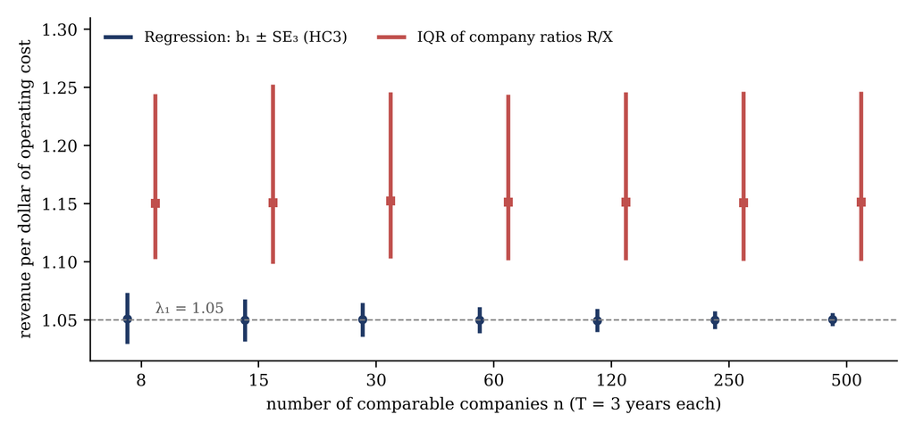
Figure 1 makes the contrast visible. It reports a Monte Carlo experiment of 1,000 samples at each size, with \lambda_0 = 40, \lambda_1 = 1.05, company scale lognormal, three years per company, and an error whose standard deviation is proportional to X. The regression interval contracts about \lambda_1. The interquartile range of the three-year ratios, computed under the regulation’s convention, settles at 1.10 to 1.25 with a median of 1.15, and stays there.
What large samples do to the leverage questions. Company size in Compustat is skewed, and the largest company retains leverage longer than the average. Table 2 reports, from the same design, the median of the largest company-year leverage and of the largest company leverage H(i). Both decline with n, at a slower pace than the average p/N. The same table reports how often one company moves the slope by more than one HC3 standard error when deleted, the intolerable boundary of the preceding post, under two specifications: least squares in levels, and least squares on the ratio form (1), which weights each company-year by the reciprocal of its scale.
| n | N | Median maximal leverage: company-year h | Median maximal leverage: company H(i) | Samples with |\Delta(i)|/\mathrm{SE}_3 > 1: levels | Samples with |\Delta(i)|/\mathrm{SE}_3 > 1: ratio form (1) |
|---|---|---|---|---|---|
| 8 | 24 | 0.276 | 0.687 | 38% | 33% |
| 15 | 45 | 0.205 | 0.531 | 38% | 11% |
| 30 | 90 | 0.184 | 0.477 | 33% | 6% |
| 60 | 180 | 0.130 | 0.339 | 31% | 2% |
| 120 | 360 | 0.105 | 0.274 | 30% | 2% |
| 250 | 750 | 0.085 | 0.218 | 19% | 0% |
Two conclusions follow. First, the small-sample objection is an objection to usual practice, and it falls on the interquartile range with equal weight: eight ratios give eight order statistics, and the regulation’s 25th percentile is the average of two of them. The regression reports the fragility; the interquartile range conceals it. Second, the answer to the objection is the one EdgarStat practice already gives: enlarge the sample and state the specification. In large samples the diagnostics confirm. In small samples they warn, and a warning is information the court is entitled to receive.
6. Diagnostics are quality control
Leamer (1983) asked econometricians to show whether an inference survives reasonable changes in its assumptions, and to distrust one that does not. The leverage boundaries answer that request in a specific form: the rule is fixed before the results are seen, each company is removed in turn, and the slope and its interval are reported every time. The Federal Judicial Center’s reference guide on multiple regression recommends the same check, observing whether the estimate changes as each data point is dropped, and identifies observations with extreme values of the explanatory variable as the likely source of influence (Rubinfeld 2011). The diagnostics are what the court’s own reference manual asks an expert to do. The interquartile range has no counterpart: it cannot ask whether one company determines its boundaries, because it estimates nothing that a company could determine.
7. The regulation’s question, answered in its own terms
The regulation asks for a range of results with stated probabilities. The comparables regression answers it at the tested party’s own operating cost X_0. The predicted revenue is \hat R_0 = b_0 + b_1 X_0, with prediction variance
\quad
(2)\qquad
\mathrm{SE}_{\mathrm{pred}}^2(X_0)=\hat\sigma^2(X_0)+[1,\; X_0]\, V_3\, [1,\; X_0]',
where V_3 is the HC3 covariance matrix of (b_0, b_1) and \hat\sigma^2(X_0) is the error variance at the scale of the tested party. A 75 percent probability above the lower limit and a 75 percent probability below the upper limit correspond to \hat R_0 \pm 0.674\,\mathrm{SE}_{\mathrm{pred}}(X_0) in large samples, where the laws of large numbers and the central limit theorem justify the normal quantile. The EdgarStat convention of one standard error, a 68 percent central interval, is wider and more conservative than the regulation’s 50 percent central band. Either way, the probability statement the regulation requires is a computed quantity, not a recited one.
8. Answers under cross-examination
Q. Is regression not far more complex than the interquartile range?
A. The regression is one straight line drawn through a scatter of points, one point for each company and year. The Court can see it on this chart. The line reports the revenue an independent company earns per dollar of operating cost, and a margin of error the opposing expert can recompute. The interquartile range appears simpler because its assumptions are not written down. It assumes that every company has zero fixed revenue; this data rejects that assumption. It discards half the companies by their profit. And it depends on the quantile formula: three conventions in common use give three different ranges on the regulation’s own example.
Q. And the leverage tests, the hat values, the deletion formulas?
A. They are quality control, written before I saw the result. I removed each company in turn and report the slope every time, on this one page. The Federal Judicial Center’s guide asks experts to perform this check. The interquartile range cannot perform it and reports no margin of error.
Q. You have eight companies, not twenty-four observations.
A. Eight companies is the usual practice, and the usual practice is the problem. With eight companies the interquartile range rests on two or three order statistics, and nobody reports how fragile they are. My practice uses a large sample, and the table shows that no single company determines the result.
Q. The regulation says the interquartile range is acceptable.
A. It says “ordinarily,” and in the same sentence it permits a different statistical method that provides a more reliable measure. I have given the Court both, side by side, with every number.
9. Conclusion
The leverage boundaries do not complicate the case for regression. They complete it. The interquartile range is a regression with an unstated restriction, an unstated quantile convention, an outcome-based trimming rule, and no error statement. The comparables regression states each of these choices and tests the ones that can be tested. Complexity that is disclosed and recomputable is the opposite of the subjectivity the Rule 702 jurisprudence condemns. The small-sample objection, for its part, describes usual practice and indicts the interquartile range first. Its remedy is the large sample, in which the laws of large numbers make the regression interval contract about the parameter and leave the interquartile range where it began.
References
Bazemore v. Friday, 478 U.S. 385 (1986). Omitted variables in a regression bear on probative weight, not admissibility (at 400).
Boltar, L.L.C. v. Commissioner, 136 T.C. 326 (2011). Daubert gatekeeping applied in the Tax Court.
Daubert v. Merrell Dow Pharmaceuticals, Inc., 509 U.S. 579 (1993). Reliability factors; cross-examination as the remedy for contested evidence (at 596).
Davidson, R., and J. G. MacKinnon (2004). Econometric Theory and Methods. New York: Oxford University Press. Consistency of least squares and of heteroskedasticity-robust covariance estimators.
Federal Rule of Evidence 702 and Advisory Committee Notes (2000 and 2023 amendments).
Huber, P. J. (1973). Robust regression: Asymptotics, conjectures and Monte Carlo. The Annals of Statistics 1(5): 799–821. Maximal leverage tending to zero as the condition for asymptotic normality of least-squares estimates.
Hyndman, R. J., and Y. Fan (1996). Sample quantiles in statistical packages. The American Statistician 50(4): 361–365. The nine sample-quantile conventions.
Kumho Tire Co. v. Carmichael, 526 U.S. 137 (1999). Gatekeeping extended to all expert testimony.
Leamer, E. E. (1983). Let’s take the con out of econometrics. American Economic Review 73(1): 31–43. Fragility of inference and the case for sensitivity analysis.
MacKinnon, J. G., M. Ø. Nielsen, and M. D. Webb (2023). Leverage, influence, and the jackknife in clustered regression models: Reliable inference using summclust. The Stata Journal 23(4): 942–982. Company-level leverage and influence; the few-clusters problem.
MacKinnon, J. G., and H. White (1985). Some heteroskedasticity-consistent covariance matrix estimators with improved finite sample properties. Journal of Econometrics 29(3): 305–325. HC3.
Rubinfeld, D. L. (2011). Reference guide on multiple regression. In Federal Judicial Center and National Research Council, Reference Manual on Scientific Evidence, 3rd ed., 303–357. Washington, DC: National Academies Press. Presentation of regression to courts; drop-one sensitivity.
Silva, E. A. (2026a). The travelled road. EdgarStat blog, November 16, 2026. https://edgarstat.com/blog/the-travelled-road/.
Silva, E. A. (2026b). Tolerable and intolerable leverage in the comparables regression. EdgarStat blog, November 2026.
U.S. Treasury Regulations, 26 C.F.R. §1.482-1(e)(2)(iii)(B)–(C) and (e)(5), Example 3.
Weisberg, S. (2014). Applied Linear Regression, 4th ed. Hoboken, NJ: John Wiley & Sons.
White, H. (1980). A heteroskedasticity-consistent covariance matrix estimator and a direct test for heteroskedasticity. Econometrica 48(4): 817–838.