Interest stripping is a tax technique where a company uses high-interest, intercompany debt to shift profits from high-tax jurisdictions to low-tax jurisdictions, by creating significant (interest related) deductible expenses for the borrowing entity of the MNE. It often falls under transfer pricing scrutiny, as tax authorities require interest rates on these loans to comply with the arm’s length principle.

The purpose of this article aims to determine the level of interest rates that a subsidiary can charge in compliance with arm’s length principle. It will invoke repeatedly Chapter 10 guidance from the OECD TP Guidelines.

The pricing of related party debt between parent/lender L and subsidiary/borrower B, that is the coupon rate on a principal amount P can proceed in two ways:

Regarding item 2, the issue now is what would be the credit rating of B as it links with that of L? One main issue here is that credit ratings of L are in practice updated infrequently. So, it makes sense, to use equity prices instead (updated frequently) to derive arm’s length coupon rates. This is the route we shall follow on the rest of this article.

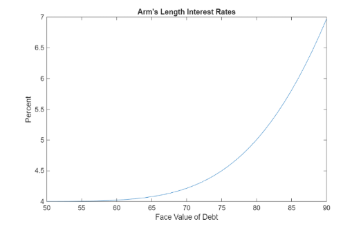
From OECD TP Guidelines, Ch. 10, we are provided with two main methods, that is the Cost Approach and the Valuation of Expected Loss Approach. Let’s consider the Cost Approach first. In employing this method, the equity value of entity E is seen as a call option on the value of the separate enity V with strike price the face value of debt D at maturity. It follows by put call parity equation (see for example, Options, Futures, and Other Derivatives by John C. Hull):

P + V = D e^{-rT} + E

Where then the market value of debt M, at time zero is given by:

M = D e^{-rT} - P = V - E

Given full implicit support, the volatility of returns of L is the same as that of B and in that case the activities of B are just a scaled version of L. Given, the market interest rate r at which L borrows from the external markets, by the realistic alternatives principle then the interest rate charged by L to B should satisfy the equation:

M = D e^{-(r+g)T}

Where g can be interpreted as the guarantee fee paid by B to L.

Below we provide an example of the above method where we have:

r = 4%

T = 1

V0 = Value of firm at time 0 = 100 million USD

sigma = Volatility of firm value = 0.2

D is the face value of debt one year from now ranging 50 million USD to 90 million USD.

Putting it all together, we get the arm’s length interest rate chargeable from L to B.

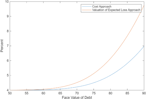
The issue here is that the interest rates computed above provide a minimum level as in reality entity can default prior to maturity if the entity value falls below a barrier H, where for simplicity we have H = (1+m)*D where m is the markup over debt that has to be satisfied for the entity to be free from bankruptcy. Here, we apply the Valuation of Expected Loss Approach. In this case, the equity becomes worthless when the value of the firm hits H and the debt holders provide a rebate of H-D to the equity holders and then taken over the firm’s proceedings. Using techniques from Hull’s book we get the following arm’s length interest rates that implicitly provide a maximum to the guarantee fee.

Lastly, we compute the range of guarantee fees as a function of leverage or debt versus equity for B. As one sees from the table as firm becomes severely levered or thinly capitalized the guarantee fee range shifts up and widens to adjust for the additional risk borne by B. Also, assuming B is at the threshold of thin capitalization, or leverage of about 3, we see that minimum guarantee fee is about 0.5% and maximum is 1.5% for example.

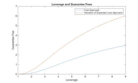
Summarizing, in this article I developed a technique for constructing an arm’s length range of guarantee fees where the Cost Approach provides the minimum and the Valuation of Expected Loss Approach the maximum values. Further, I observe that as leverage of the borrowing entity increases, the risk of the firm going bankrupt increases and this translates into a uniform upward shift in the arm’s length range for guarantee fees together with a widening of the range. The main assumption holding all together is that of full implicit support where it is assumed the activities of the borrower and lender are very highly interlinked, so their activities are scaled versions of one another.

References

1. OECD Transfer Pricing Guidelines for Multinational Enterprises and Tax Administrations, January 2022.

2. Options, Futures, and Other Derivatives, 11e, by John C. Hull.