Introduction

When applying the Comparable Profits Methods (CPM), Return on Assets (ROA) is often used as a Profit Level Indicator (PLI) to establish, in principle, the arm’s length price for a related party transaction. In general, this PLI is given by:

{ROA} = \frac{{Operating Income}}{{Operating Assets}}

In practice, the arm’s length range for ROA for a tested party is determined via an interquartile range (IQR) derived from the ROAs of comparable companies, which in turn are derived from a functional analysis. However, the IQR is a non-parametric summary of the central half of the data. Whether it yields a reliable arm’s length range depends on how well the structural equation describing profit drivers reflects reality. When using the interquartile range, one assumes that:

Operating Income
= \beta \times Operating Assets
+ residual

where the residual has the usual properties of mean zero, and so on. In general, though, Operating Income (OI) is driven by other factors besides Operating Assets (OA) and in this article we shall describe a straightforward economic model of an industry where two main factors drive OI, that is 1) OA and 2) an expected term regarding future profitability which depends on whether currently the industry experiences good or bad times. The presence of 2) implies that median ROA and ranges as measured by running the vanilla approach are biased estimates and, as such, underreport or overreport relative to the true arm’s length values.

A Fully Fledged Economic Model

Consider a market with n firms, where each firm faces a constant marginal cost c, with market demand:

Q = a - b \times p

Suppose each firm faces a Weighted Average Cost of Capital (WACC), which translates into a discount factor 𝛿 for each firm. The firm operates in time periods t = 0, 1, 2, …. Each period an aggregate shock a occurs with aL occurring with probability q and aH with probability 1-q.

Each firm employs a reward-and-punishment pricing strategy. That is, if all goes according to plan each firm sets price pL in bad times and pH in good times. However, each firm can also deviate by setting a price slightly lower than the rest and capturing all the market share. In case of deviation, each remaining firm sets its price equal to c or marginal cost, with future operating profits set to zero.

It has been shown by Rotemberg and Saloner (1986) that for a discount factor satisfying:

\delta \ge \frac{n - 1}{n - q}

each firm sets the monopoly price pL in bad times and the monopoly price pH in good times and produces QL/n and QH/n, respectively. In return, the firm earns monopoly profit πL/n in bad times and πH/n in good times.

Using methodology, say from Copeland, Weston and Shastri (2014), one can also deduce the OA in good and bad times for each firm. It follows then, in bad times we have πL/n = π* and in good times πH/n = π**, given by:

\pi^* = (1 - \delta)\, OA^* - \delta (1 - q)\, \frac{\Delta}{n}

\pi^{**} = (1 - \delta)\, OA^{**} + \delta q\, \frac{\Delta}{n}

The two equations above provide a structural specification of the evolution of profits in good and bad times, with drivers: OA of the firm and a weighted profit differential, which is negative in bad times and positive in good times, quantified by Δ = π_H – π_L.

Monte Carlo Simulation

Suppose that the above equations determine profits based on the background structural model. We shall then proceed to conduct the following experiment.

1. Run a binary random number generator to simulate a over 30 periods.

2. Calculate resulting profits and compute OA simultaneously.

3. Run the regression: OI = β OA + residual and collect an estimate of beta or β*

4. Repeat 1 through 3, say 20 times.

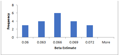
From the above, true β = (1-δ). However, when we run the above experiment, we obtain a sampling distribution of beta estimates. For a specific parameterization of the model by aL = 9, aH = 11, b = 1, c = 4, p = 0.3, we get the following sampling distribution with a mean of 0.066 and a lower range of 0.06, while a higher range of 0.072. On the other hand, the true beta is 0.074. From this simulation, one can see that the interquartile range would underreport the true ROA by approximately 1%.

Reference

1. A Supergame-Theoretic Model of Price Wars during Booms
   Author(s): Julio J. Rotemberg and Garth Saloner
   Source: The American Economic Review, Vol. 76, No. 3 (Jun., 1986), pp. 390-407

2. Financial Theory and Corporate Policy, Fourth Edition
   Author(s): Thomas E. Copeland, J. Fred Weston and Kuldeep Shastri
   Source: Pearson Education Limited