Tutorial: Power Functions in Transfer Pricing

A power function has the form: 

(1) Y = X ^β 

where the slope parameter β is determined from data comparable to the tested party. Y is the dependent variable and X is the independent (explanatory or predictor) variable.

The contrived linear function: Operating Profits = β Revenue, with the forced zero intercept specified in the U.S. and OECD guidelines, and the quadratic and cubic functions are power functions. Other power functions include the reciprocal and squared-root functions. 

Typical power functions in economics include: 

1. Linear: Y = β X, like the U.S. and OECD profit indicators. 
2. Quadratic: Y = X ², where β = 2. 
3. Cubic: Y = X ³, where β = 3. 
4. Reciprocal: Y = 1 / X, where β = −1. 
5. Squared root: Y = √ X = X ^1/2, where β = 1/2.  

Here, we examine a power function that is prevalent in economics: 

(2) Y = α X ^β 

and take the first derivative of (2) to obtain the slope coefficient: 

(3) d Y / d X = β α X ^{β – 1} 

Slope = β α (X ^β / X) = β (Y / X)

Except for the special case in which α = β = 1, we can use the double-logarithms regression to estimate the slope of the power equation (2): 

(4) LN(Y) = LN(α) + β LN(X) 

Now, we consider the best regression fit among two rival operating profits functions using actual company-level annual data: 

(5) Y = α + β X,

versus the power equation (2) or its regression version (4). 

Chart 1 contains the linear regression: Y = 0.071 X, with the Newey-West t-statistics of the slope = 7.8158 and the R² = 0.8032. The alpha-intercept is not significant, so we don’t report it. 

Chart 1: Linear Regression

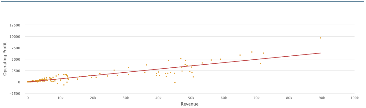
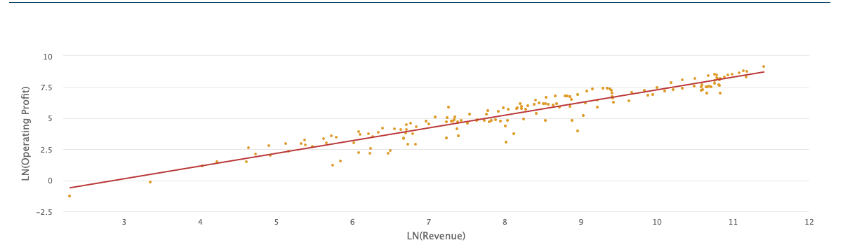
Chart 2 contains in this case a superior (more reliable) double-logarithms regression (4): LN(Y) = 1.0219 LN(X) − 2.938, with the Newey-West corrected t-statistics of the intercept = − 8.6162, the t-statistics of the slope coefficient = 26.035, and the R² = 0.9043. Each regression contains 167 annual paired X and Y observations. 

Chart 2: Double-Logrithms Regression 

As takeaway, we must examine the comparable company data using bivariate scatterplots instead of assuming the special (contrived) linear equation without an intercept: 

(6) Y = β X,

where the intercept of linear function (6) is forced to be α = 0. 

The regression results above were computed online in EdgarStat using the historical pairs of X = Revenue (REVT) and Y = Operating Profits (OIADP) of five U.S. retailers :  

1. 73119 Bed, Bath & Beyond (BBBY), 1990-2021 
2. 27050 Best Buy Inc. (BBY), 1983-2021 
3. 107748 Conn's Inc. (CONN), 2000-2021 
4. 5067 Lowe’s Companies Inc. (LOW), 1984-2021 
5. 36090 Williams Sonoma Inc. (WSM), 1986-2021