In current practice, the profit indicator under the CPM (TNMM) is calculated in four steps:
- Select the comparables to the tested party (taxpayer).
- Select the profit indicator.
- Calculate quartiles of the profit indicator.
- Determine if asset adjustments to the profit indicator are significant.
The problem with these four steps is that the calculation of quartiles depends on special assumptions: First, the relationship between the profit indicator and the base (revenue, total cost, or assets) is linear; second, the intercept is insignificant.
In addition, there is no direct way to test the effects of assets employed on the profit indicator. As a result, the interquartile range of the profit indicator is wide (unreliable), and the asset intensity adjustments are ad hoc (arbitrary, without economic merit).
These problems can be solved by using regression analysis, which produces more defensible statistical ranges of the profit indicator that are more resistant to audit scrutiny.
However, estimating structural equations like the underlying linear equation of quartiles produces biased (omitted variable) results. Therefore, I suggest using the reduced-form equation:
(1) R(t) = C(t) + Y(t)
(2) Y(t) = α + β R(t) + U(t)
R(t) = α + C(t) + β R(t) + U(t)
R(t) − β R(t) = α + C(t) + + U(t)
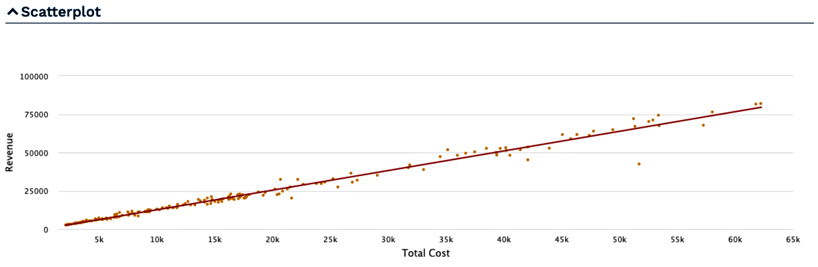
(3) R(t) = λ0 + λ1 C(t) + V(t)
where the intercept λ0 = α / (1 – β) and the slope coefficient λ1 = 1 / (1 – β) > 1 is the operating profit markup.
The operating profit margin can be obtained by solving for β from λ1:
(4) λ1 = 1 / (1 – β) ⇔ β = (λ1 – 1) / λ1
The necessary variables per company to estimate the reduced-form equation (3) can be found in EdgarStat®:
(a) R(t) is revenue in year t = 1 to T audit years (plus at least two prior or post audit years).
(b) C(t) is total cost, which is the sum of direct cost and indirect expenses (including depreciation and amortization). Thus, the indirect least squares slope coefficient β is the operating profit margin after depreciation and amortization (EBIT margin).
(c) Y(t) is operating profit after depreciation and amortization (EBIT).
(d) The unknown variables U(t) and V(t) are the random uncertainty.
Example from five U.S. pharmaceutical companies (annual data from 1982 to 2019):
| Company | Count | λ1 | t-Statistics | R2 | Intercept (λ0) |
| Abbott Laboratories | 38 | 1.1616 | 41.1 | 0.992 | Significant (2.4) |
| Bristol-Myers Squibb | 38 | 1.2645 | 59.3 | 0.9669 | Insignificant |
| Johnson & Johnson | 38 | 1.35 | 87.3 | 0.9964 | Insignificant |
| Eli Lilly | 38 | 1.1589 | 21.5 | 0.9603 | Significant (2.2) |
| Pfizer | 38 | 1.2496 | 58.5 | 0.9868 | Insignificant |
| All | 190 | 1.2976 | 65.5 | 0.9897 | Insignificant |
The OLS (ordinary least squares) regression results above can be computed in EdgarStat online (interactive applications) using the Scatterplot or the Regression function.
The Newey-West t-statistics correct for autocorrelation among the regression residuals. See https://www.econometrics-with-r.org/15.4-hac-standard-errors.html