
Introduction
Consider the uniform distribution of a random variable Y with support from 0 to b. Its mean is 0.5b yet the mean is just a moment of the distribution – it’s a measure its central tendency. Yet, to get a more complete picture of the distribution, we can consider certain locations of the distribution. That is one can ask:
- What is the value of y in the distribution such that Prob (Y <= y) = κ? Denote that value by QY(κ).
The answer to the above is obviously QY(κ) = κb. Hence, QY(0.25) = 0.25b which is the lower quartile. Also, QY(0.5) = 0.5b is the median and QY(0.75) = 0.75b is the upper quartile. The core idea though, is that for a quantile κ, 100κ percent of the distribution is to the left of κb and 100(1-κ) is to the right of κb.
In a similar vein, quantile regression is to OLS regression what quantiles are to the mean in terms of describing locations of a distribution1. Quantile regression is a statistical analysis that can be used to approximate the whole conditional distribution of a response variable given a set of explanatory variables and therefore does not restrict attention only to the conditional mean like least squares regression. That is for a given κ, quantile regression can be used to identify the regression line where 100κ percent of the response variable is below the line, and 100(1-κ) percent is above the line. Quantile regression could be an added useful tool alongside OLS as a valid statistical method in transfer pricing. Yet its usefulness has still to be verified.
Quantile Regression Applied To Transfer Pricing
Let’s consider an industry where for a firm j the following accounting identity holds:
OIBDP_j = REVT_j - XOPR_j
where REVT is net sales or revenue and XOPR equals COGS + XSGA per the glossary in EdgarStat.
Let’s also consider the revenue generating function:
REVT_j = \alpha_0 + \alpha_1 XOPR_j + \epsilon_j
where we have:
VAR(\epsilon_j) = \alpha_2^2 XOPR_j^2
In this formulation, the error term is heteroscedastic and the variance of revenue increases in scale with increases in XOPR which is observed in the data.
Rearranging the two equations above:
OIBDP_j = \alpha_0 + (\alpha_1 - 1) XOPR_j + \epsilon_j
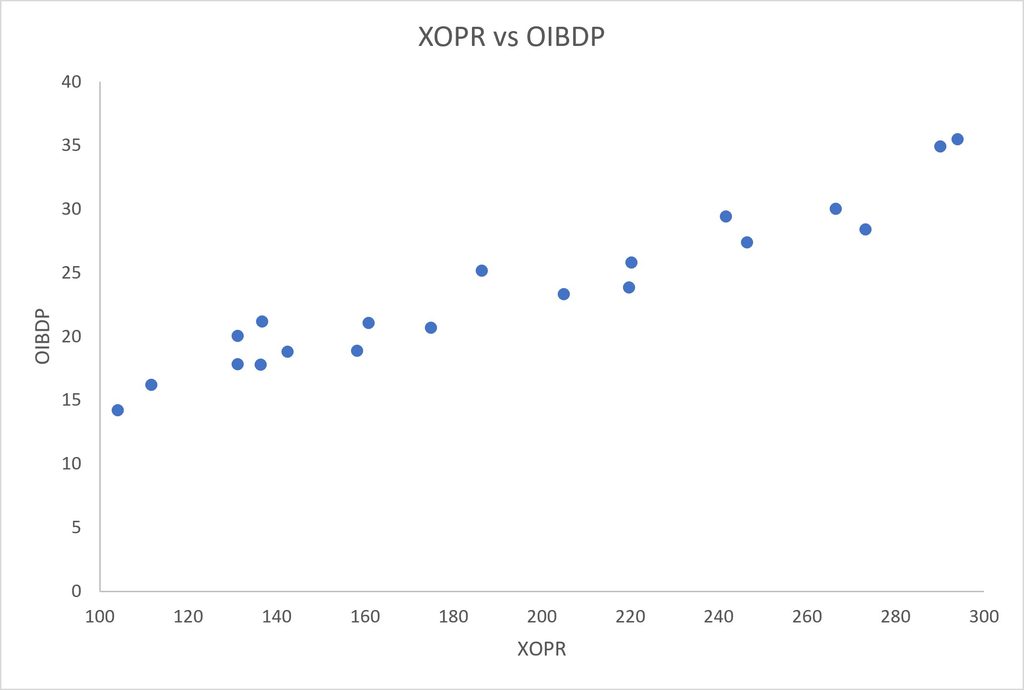
We first simulate N=20 values for XOPR by picking randomly using numpy package in Python from a uniform distribution with support 100 to 300. Given XOPR, we pick the following parameterization:
\alpha_0 = 5.00
\alpha_1 = 1.10
\alpha_2 = 0.01
Given the above parameterization, we use the above generating function for OIBDP to obtain 20 data values. The following graph below summarizes this process:
We then use the Python statsmodels package to obtain coefficient estimates for the 25th, 50th, 75th and the OLS regression with robust HC3 errors. The following graph illustrates the regression lines.
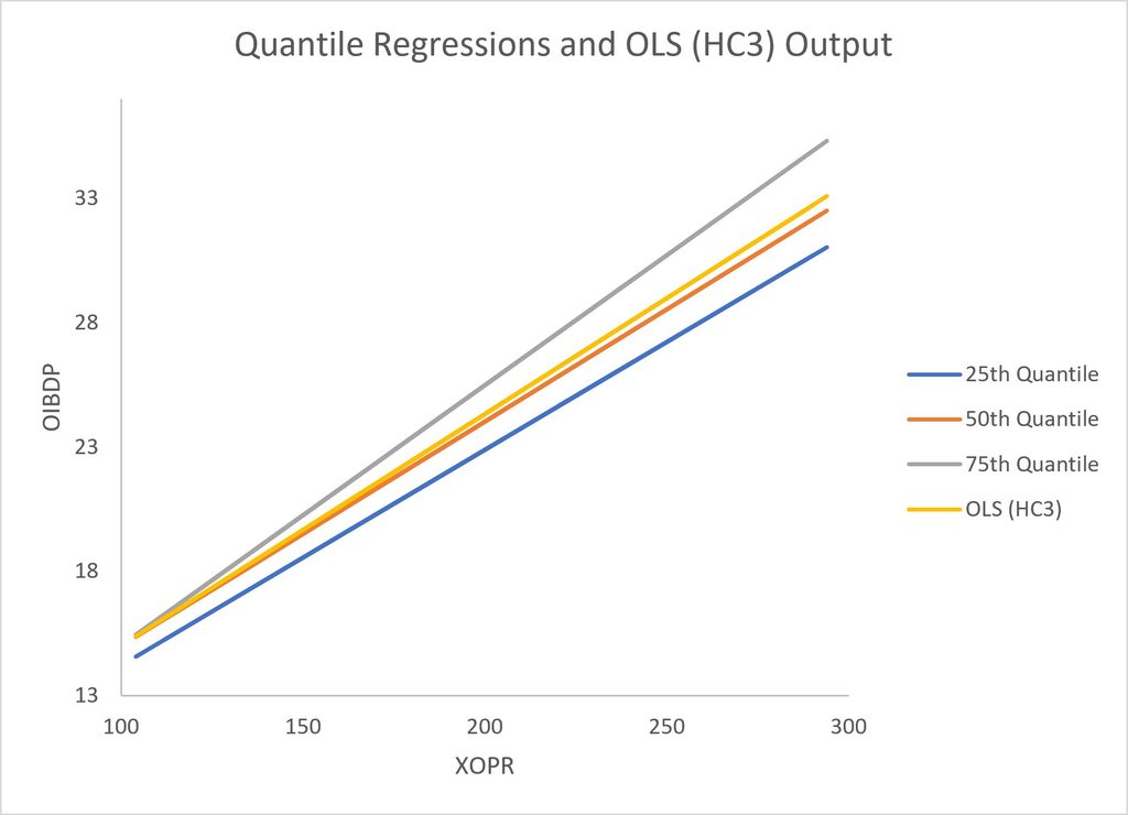
In transfer pricing we are interested in whether we can show a reliable range for the profit level indicator of interest. In this case, the profit level indicator of interest is Markup Over Total Cost (MOTC) = α1 – 1. Using the inference properties of quantile regression and OLS we obtain the following summary:
| Regression | MOTC^ | St Error (MOTC^) | Pseudo R2 / R2 |
| 25th | 0.0868 | 0.015 | 0.7198 |
| 50th | 0.0904 | 0.013 | 0.7340 |
| 75th | 0.1047 | 0.016 | 0.7367 |
| OLS (HC3) | 0.0933 | 0.008 | 0.9240 |
From this simple exercise we see that the standard error of the coefficient estimate for OLS is lowest amongst four even considering the case of HC3 errors. The OLS (HC3) 68% confidence interval for the coefficient estimate is (0.853, 0.1013) and includes the true population coefficient of 0.1. The Euclidean distance of the established range is 0.016.
One can also show a range by considering instead the interval (0.0868, 0.1047). The Euclidean distance is 0.0179. Both intervals contain the population coefficient of course and they overlap. Or one could take the 50th quantile regression coefficient estimate and show a range around it that also contains the population coefficient, that is (0.0774, 0.1034). The latter constructs do not provide a tighter range than OLS.
Conclusion
It does not seem from the context of this simulation with heteroscedastic errors that there is much to be gained by using quantile regression over OLS (HC3) in terms of establishing an arm’s length range for the PLI of interest. However, we can use quantile regression to corroborate the results of OLS combined with HC3 standard errors.
References
- Cristina Davino, Marilena Furno and Domenico Vistocco, “Quantile Regression: Theory and Applications”, John Wiley and Sons, Ltd, 2014.